Variational Autoencoder

What is Variational Autoencoder?

From AE to VAE

VAE is a generative model. VAE is aimed to build a model that generates data similar to that of $X$ in the training database.

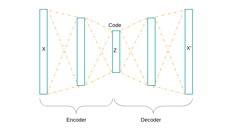
Consider the autoencoder. Autoencoder does not care about the $z$’s structure. AE just encrypts the data and decrypt afterward.

However, in order to generate data, we need more firm control over the space of $z$’s. In other words, we want $p(z)$ of our autoencoder to follow certain distribution which is really familiar to us (e.g. Gaussian). This is what VAE does.

Latent vector $z$

Here is the first checkpoint. Here we assume that there exists a vector $z$ that inherits all the properties of $X$.

For variable $z$, we call it “Latent”. “Latent” is just a fancy way of calling “hidden” - this $z$ “hides” every tedious details of $X$ and gives us the essence of it.

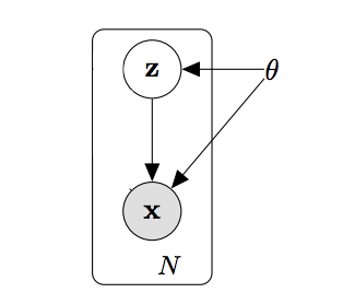
$z$ contains the essence of $x$, and that can decide what x is.

Here, we are interested in the value of $ P(z|X) $, which we call the posterior distribution. This gives the probability of latent variable $z$ given the evidence $X$. If we get to know this, we can feed $X$ to our encoder network and this network will give $z$ as an output.

$z$’s are intractable

In order to calculate the posterior $ P(z|X) $, we need to set up the formula with respect to every possible $z$’s.

Here, using the bayesian rule would be a good choice.

$ P(z|X) = \frac{P(X|z) P(z)}{P(X)} $

Technically, $P(X|z)$ is called the likelihood and $P(z)$ is called the prior distribution (and our objective was to make this prior to follow desired distributions).

For the denominator, P(X) can be calculated with respect to all possible values of $z$’s. That is,

$P(X) = \int\limits_{z} P(X|z) P(z) ,dz$.

However, integrating over $z$ is hard, as there are too many $z$’s possible out there.

For example, if we only pick $z$’s dimension as 2, any points in the whole 2D plane correspond to $z$’s possible value.

We say this integral is “intractable”. Most of $z$’s would not produce the data that we want, which means $p(z) = 0$ for most of the time.

Bayesian Inference

What can we do then? Here’s where bayesian inference comes.

We try to approximate $P(z|X)$, not exactly to calculate.

This can be done by setting another distribution $Q(z|X)$, and pull $Q(z|X)$ to $P(z|X)$ as much as possible.

KL-divergence

Difference of the two distributions $Q(z|X)$ and $P(z|X)$ can be calculated using KL-divergence.

For probability distribution A and B, we define KL divergence of B with respect to A as:

$D_{KL}[A(\theta)||B(\theta)] = E_{\theta \sim A}[log(\frac{A(\theta)}{B(\theta)})] = E_{\theta \sim (A)}[log(A(\theta)) - log(B(\theta))] $

Similarly, KL divergence of $Q(z|X)$ with respect to $P(z|X)$ is as follows:

$D_{KL}[Q(z|X) || P(z|X)] = E_{z \sim Q(z|X)}[log Q(z|X) - logP(z|X)] $

And by fixing $P(z|X)$ using bayesian rule:

$= E_{z \sim Q(z|X)} [log Q(z|X) - log(\frac{P(X|z) logP(z)}{logP(X)}) ] $

$= E_{z \sim Q(z|X)}[log Q(z|X) - log(P(X|z) - logP(z) + logP(X)] $

$= E_{z \sim Q(z|X)}[log Q(z|X) - log(P(X|z) - logP(z)] + logP(X) (\because\ logP(X)\ is\ nothing\ to\ do\ with\ z) $

$= - E_{z \sim Q(z|X)}[log(\frac{P(X|z)P(z)}{Q(z|x)})] + logP(X)$

ELBO

Until here, we have:

$D_{KL}[Q(z|X) || P(z|X)] = - E_{z \sim Q(z|X)}[log(\frac{P(X|z)P(z)}{Q(z|x)})] + logP(X) $

Rearranging with respect to $logP(X)$, we have:

$logP(X) = D_{KL}[Q(z|X) || P(z|X)] + E_{z \sim Q(z|X)}[log(\frac{P(X|z)P(z)}{Q(z|x)})] $

Let’s analyze term by term.

On RHS, we have $logP(X)$. This term is constant.

On LHS, we have two terms.

First term is $D_{KL}[Q(z|X) || P(z|X)]$ and this was our objective, KL term to minimize.

Second term is $E_{z \sim Q(z|X)}[log(\frac{P(X|z)P(z)}{Q(z|x)})]$.

Here’s the important point.

As RHS is constant, our objective of minimizing KL term can be done by maximizing the second term, $E_{z \sim Q(z|X)}[log(\frac{P(X|z)P(z)}{Q(z|x)})]$.

This term is usually called ELBO (Evidence Lower Bound) term.

Our Loss term using ELBO

Since our objective has changed to Maximizing ELBO, let’s analyze that term.

Here’s our ELBO term:

$E_{z \sim Q(z|X)}[log(\frac{P(X|z)P(z)}{Q(z|x)})]$

This term can be separated into two by following:

$= E_{z \sim Q(z|X)}[log(P(X|z) + log(\frac{P(z)}{Q(z|x)})]$

$= E_{z \sim Q(z|X)}[log(P(X|z)] + E_{z \sim Q(z|X)}[log(\frac{P(z)}{Q(z|x)})]$

$= E_{z \sim Q(z|X)}[log(P(X|z)] - D_{KL}[Q(z|X)||P(z)]$

What are these two terms?

First term, $E_{z \sim Q(z|X)}[log(P(X|z)]$, corresponds to Log likelihood. Maximizing ELBO leads to maximizing log likelihood of decoder output $X$ given encoder output $z$.

Second term, $ D_{KL}[Q(z|X)||P(z)]$, corresponds to KL divergence of $Q(z|X)$ and $P(z)$. Maximizing ELBO means maximizing negative of this KL, and this leads to minimizing this KL term. Intuitive explanation for this work is “Make the output of encoder network is similar to that of our prior $p(z)$”.

Combining those two, our objective of “Maximizing ELBO” has become:

Maximize the log likelihood of decoder output, while making the output of encoder network is similar to that of our prior $p(z)$.

Congrats! Now our network perfectly follows our objective!

Optimization

For our neural net, let’s make our objective into minimizing the negative of ELBO rather than maximizing ELBO.

Slight change in our objectives are, minimizing the negative log likelihood and KL term of encoder network and our prior.

$ Minimize\ Loss = Negative Log Likelihood + KL(encoder, prior) $

Assumptions on Data Distribution (Negative Log Likelihood)

If our data $X$ follows Gaussian, our Negative Log Likelihood becomes Mean Squared Error (MSE) Loss.

If our data $X$ follows Categorical distribution, our Negative Log Likelihood becomes Cross Entropy (CE) Loss.

Assumptions on Prior (KL term)

If our prior and our encoder network are assumed to follow Gaussian, our KL term has analytical solution. That is:

$ D[N(\mu_0, \Sigma_0)||N(\mu_1, \Sigma_1)] = \frac{1}{2}(tr(\Sigma_1^{-1}\Sigma_0) + (\mu_1 - \mu_0)^{T}\Sigma_1^{-1}(\mu_1 - \mu_0)-k+log(\frac{det\Sigma_1}{det\Sigma_0}) $

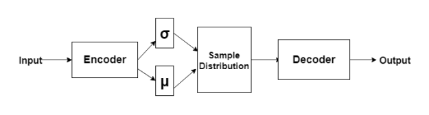
Final Architecture

The final architecture of VAE is as follows. Well done!

---

This is the 2nd draft written on Oct 10, 2021

2nd draft: 2021-10-10

1st draft: 2021-10-03