
Cobweb Process Modeling with Python
Updated:
The task is to devise a model representing Cobweb Process.
Python is used for representation.
Modeling:
Let’s model the cobweb process into code.
Let’s install additional package first: pynverse.
This package is used to get inverse function.
Why?
In economic modeling, price P, the independent variable is usually located vertical axis, not horizontal axis.
!pip install pynverse
Let’s import the setups.
import matplotlib.pyplot as plt
import numpy as np
from pynverse import inversefunc # this package provides inverse function
Firstly, Let’s define the function to plot market status, plotMarket.
def plotMarket(D, S, Q_max, P_max):
	# ranges to plot
	plt.xlim(left = 0)
	plt.xlim(right = Q_max)
	plt.ylim(bottom = 0)
	plt.ylim(top = P_max)

    # create list for prices.
    rangeP = np.linspace(0, P_max, P_max * 100)

    # plot Demand/Supply curves, using price range
    plt.plot(list(map(D, rangeP)), rangeP)
    plt.plot(list(map(S, rangeP)), rangeP)
In here, plotMarket gets 4 parameters
- D, S: functions(lambda) representing Demand and Supply Curve
- Q_max, P_max: representing maximum range of the coordinate
And also, let’s setup a function which draws line between two points, connectPoints.
def connectPoints(point1, point2):
    plt.plot([point1[0], point2[0]],[point1[1], point2[1]] , 'k-', linewidth = 1)
In here, connectPoints gets 2 parameters representing coordinates, by a list.
Next, let’s devise a cobweb process.
def cobwebProcess(D, S, S_adj, init_price, ϵ, periods):
    P = init_price
    S_inv = inversefunc(S)

    for i in range(periods):
        S_cur = [S(P), P]
        D_cur = [D(P), P]
        connectPoints(S_cur, D_cur)
        # Supplier is adjusting Quantity, according to current demand
        Q = S_adjusting_function(D(P))
        P = S_inv(Q)
        S_next = [Q, P]
        connectPoints(D_cur, S_next)

        # if market is near equilibrium, break.
        if(abs(D(P) - S(P)) < ϵ):
            print("Market is in equilibrium.\n",\
                  "Iteration: ", i+1, "\n",\
                  "-Supply side\n",\
                  "P: ", P, "\n",\
                  "Q: ", S(P), "\n", \
                  "-Demand side\n",\
                  "P: ", P, "\n",\
                  "Q: ", D(P), "\n", \
                 )
            break

        # if market was not able to reach equilibrium, report.
        if((i == periods - 1) and (abs(D(P) - S(P)) >= ϵ)):
            print("Economy wasn't able to reach equilibrium.\n",\
                  "-Supply side\n",\
                  "P: ", P, "\n",\
                  "Q: ", S(P), "\n", \
                  "-Demand side\n",\
                  "P: ", P, "\n",\
                  "Q: ", D(P), "\n", \
                 )
In here, plotMarket gets 6 parameters
- D, S: functions(lambda) representing Demand and Supply Curve
- S_adj: functions(lambda) representing suppliers’ adjusting behavior. How would suppliers’ react to unexpected, wrong “quantity demanded”?
- init_price: as it’s name suggests!
- ϵ: epsilon, which meant to be admissible error. If we can get the situation of S(Q) = S(D), it would be perfect. However, it is sometimes impossible because of market status, or by technical problem.
- periods: This represents how many iterations or process being done.
Let’s do the setup first.
P = init_price
S_inv = inversefunc(S)
And in iteration, we have,
S_cur = [S(P), P]
D_cur = [D(P), P]
connectPoints(S_cur, D_cur)
# Supplier is adjusting Quantity, according to current demand

Q = S_adjusting_function(D(P))
P = S_inv(Q)
S_next = [Q, P]
connectPoints(D_cur, S_next)
We now have current status of market as : S_cur, D_cur
If the economy is not in equilibrium, what would be the supplier’s response?
According to our model, given D(P), supplier would respond as supplying S_adjusting_function(D(P)).
Let’s experiment few examples of adjusting function later on!
Anyway, by that adjustment, next periods’ supply is determined. Here, S_next.
Next, we can define equilibrium condition as abs(D(P) - S(P)) < ϵ, which means quantity supplied and quantity demanded are almost identical.
If we are near equilibrium, break. report.
# if market is near equilibrium, break.

if(abs(D(P) - S(P)) < ϵ):
	print("Market is in equilibrium.\n",\
        "Iteration: ", i+1, "\n",\
        "-Supply side\n",\
        "P: ", P, "\n",\
        "Q: ", S(P), "\n", \
        "-Demand side\n",\
        "P: ", P, "\n",\
        "Q: ", D(P), "\n"\
       )
  break
else, just report.
# if market was not able to reach equilibrium, report.

if((i == periods - 1) and (abs(D(P) - S(P)) >= ϵ)):
    print("Economy wasn't able to reach equilibrium.\n",\
                "-Supply side\n",\
                "P: ", P, "\n",\
                "Q: ", S(P), "\n", \
                "-Demand side\n",\
                "P: ", P, "\n",\
                "Q: ", D(P), "\n", \
                )
Case Study:
Let’s do some case analysis.
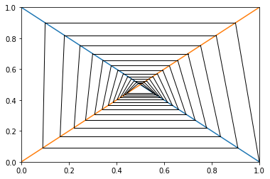
Case 1
$ D: Q = 1 - P $
$ S: Q = P $
$ Adj: Q_{n+1} = D^{-1}(P_n) * 0.9 $
$ P_0 = 0 $
D = lambda P: 1-P
S = lambda P: P
S_adjusting_function = lambda Q: 0.9* Q
init_price = 0
Q_max = 1
P_max = 1
plotMarket(D, S, Q_max, P_max)
cobwebProcess(D, S, S_adjusting_function, init_price, 0.01, 100)
plt.show()
Result for case 1:
Market is in equilibrium.
 Iteration:  27
 -Supply side
 P:  0.5012288227909136
 Q:  0.5012288227909136
 -Demand side
 P:  0.5012288227909136
 Q:  0.49877117720908637
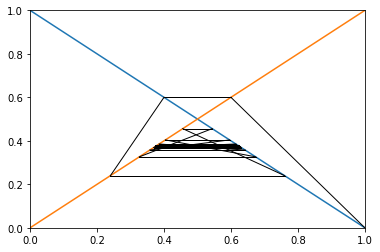
case 2
$ D: Q = 1 - P $
$ S: Q = P $
$ Adj: Q_{n+1} = D^{-1}(P_n) * 0.6 $
$ P_0 = 0 $
D = lambda P: 1-P
S = lambda P: P
S_adjusting_function = lambda Q: 0.6 * Q
init_price = 0
Q_max = 1
P_max = 1
plotMarket(D, S, Q_max, P_max)
cobwebProcess(D, S, S_adjusting_function, init_price, 0.01, 100)
plt.show()
Result for case 2:
Economy wasn't able to reach equilibrium.
 -Supply side
 P:  0.37499999999999994
 Q:  0.37499999999999994
 -Demand side
 P:  0.37499999999999994
 Q:  0.625
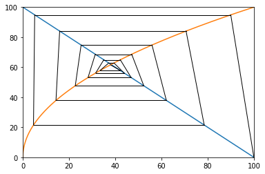
case 3: Square Supply
$ D: Q = 100 - P $
$ S: Q = \frac{ P^2 }{100} $
$ Adj: Q_{n+1} = 0.9 * D^{-1}(P_n) $
$ P_0 = 0 $
D = lambda P: 100-P
S = lambda P: (P**2)/100
S_adjusting_function = lambda Q: 0.9 * Q
init_price = 0
Q_max = 100
P_max = 100
plotMarket(D, S, Q_max, P_max)
cobwebProcess(D, S, S_adjusting_function, init_price, 1, 100)
plt.show()
Result for case 3:
Market is in equilibrium.
 Iteration:  13
 -Supply side
 P:  61.58917120536864
 Q:  37.9322600976421
 -Demand side
 P:  61.58917120536864
 Q:  38.41082879463136
Code in jupyter notebook is available at my github.
Leave a comment